Solving Handwritten Equations with Deep Learning

In today’s digital age, machine learning (ML) has revolutionized numerous fields, including image recognition and natural language processing. One intriguing problem that combines both these areas is the automatic solving of handwritten mathematical equations. Imagine taking a picture of a complex equation and having a machine instantly provide the solution. This blog post delves into how I built a machine learning model to achieve just that.

Problem Statement

The task at hand is to develop a system that can take an image of a handwritten mathematical equation and output the correct answer.

To tackle this, the problem can be broken down into two primary components:

• Reading and detecting the symbols: The system must recognize individual numbers and mathematical symbols from the image.
• Solving the equation: Once the symbols are identified, the system must correctly interpret and solve the equation.

Symbol Detection with Convolutional Neural Networks (CNNs)

The first step is to accurately recognize the symbols in the image. We’ll use a Convolutional Neural Network (CNN) for this purpose, as CNNs are particularly effective for image classification tasks.

Code Blocks

Target Classes: We consider the following symbols and functions for our model:

classes_ideal = ['(', ')', '+', '-', '0', '1', '2', '3', '4', '5', '6', '7', '8', '9', '[', ']',
'cos', 'e', 'forward_slash', 'log', 'pi', 'sin', 'sqrt', 'tan', 'times']

These symbols cover a broad range of arithmetic operations and functions commonly used in mathematical equations.

Dataset

For the dataset, I used a publicly available dataset on Kaggle. You can find the dataset here .

Analyzing the dataset, we noticed an imbalance in the number of images per class. For instance, some classes like ( and ) had only 700 images, while others like 1, 2, and 5 had a significantly larger number of images.

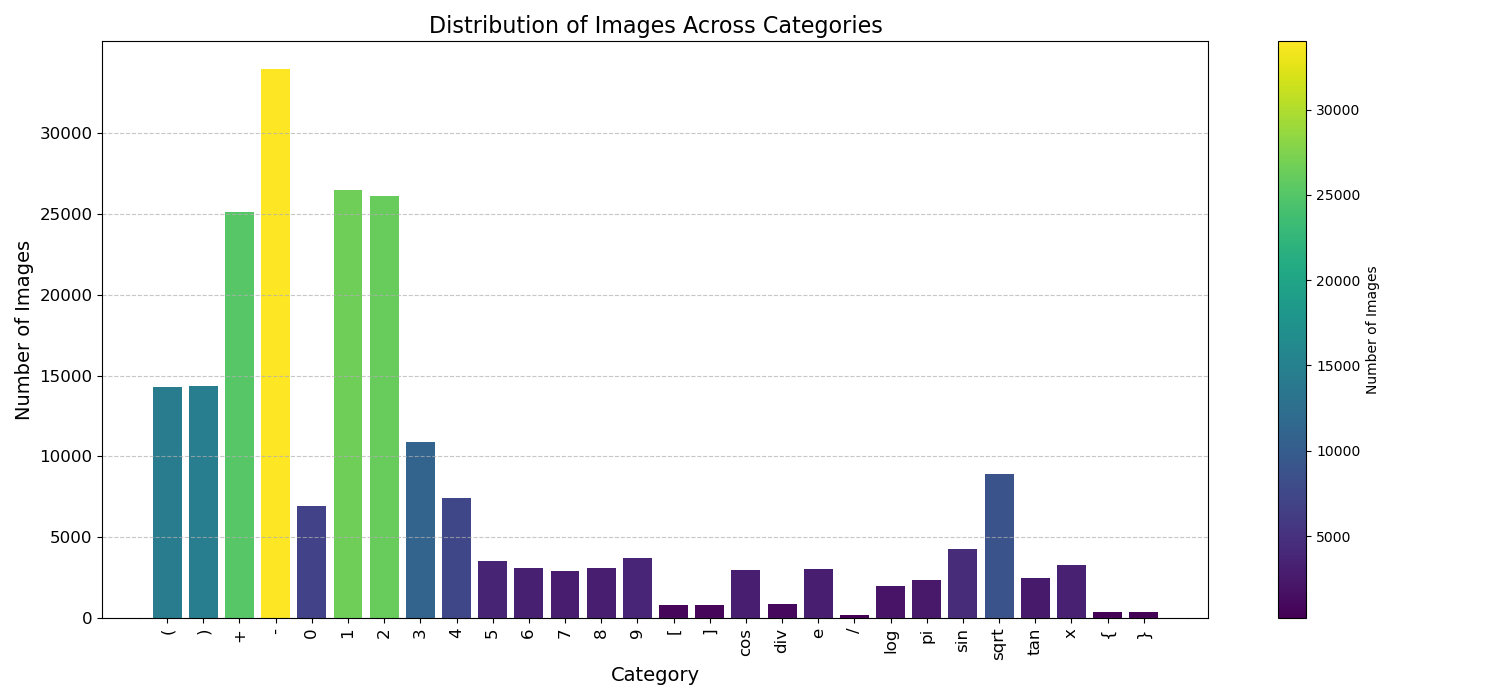
To address this imbalance, we applied data augmentation techniques to increase the number of images for underrepresented classes.

Data Augmentation

Using the ImageDataGenerator from TensorFlow, we augmented our data with the following parameters:

datagen = ImageDataGenerator(
zoom_range=[0.94, 1.5],
width_shift_range=0.09,
height_shift_range=0.09,
fill_mode='constant',
cval=255,
channel_shift_range=70.0,
)

For certain symbols like /, we generated 10 new images from each original image, whereas for others, we generated 2 new images from each.

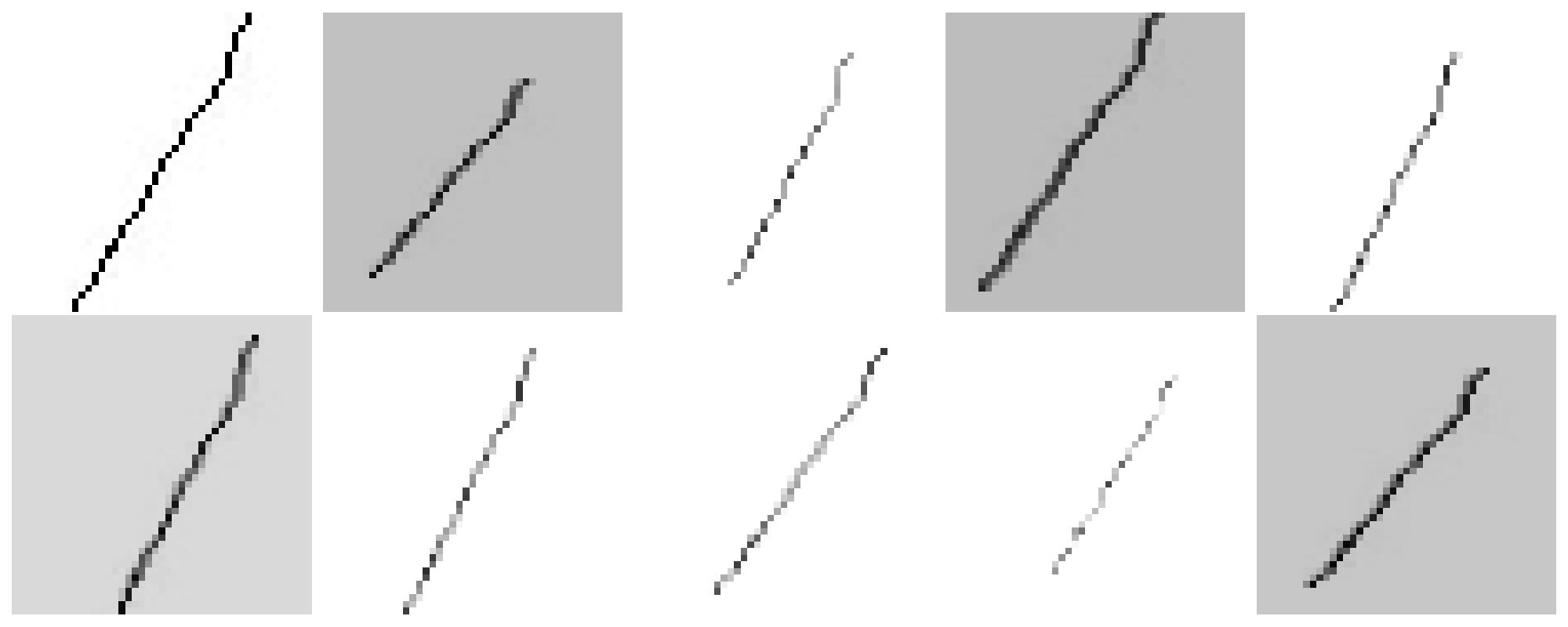
Image Preprocessing

Images were resized and converted to grayscale before being fed into the model:

def load_image(file_path, label):
image = tf.io.read_file(file_path)
image = tf.image.decode_jpeg(image, channels=3)
image = tf.image.resize(image, (45, 45))
image = tf.image.rgb_to_grayscale(image)
return image, label

Model Architecture

The CNN model was designed with several convolutional layers, followed by dense layers for classification. Here are some key terms and parameters used in our model:

• Convolutional Layer: Applies convolution operations to the input, extracting features.
• Filter, Padding, Kernel Size, Strides, Activation: Key parameters for convolutional layers.
• Flatten Layer: Converts the 2D matrix data to a vector.
• Dense Layer: A fully connected layer for classification.
• Kernel Initializer, Regularization, Dropout: Techniques to prevent overfitting and improve generalization.
• Optimizer, Loss Function: Used for training the model.

Here is the architecture of the CNN model:

model = Sequential([
keras.Input(shape=(45, 45, 1)),
Rescaling(1./255),
Conv2D(32, (3, 3), strides=(1, 1), padding='same', activation='relu',
kernel_initializer='glorot_uniform', bias_initializer='zeros'),
Conv2D(32, (3, 3), strides=(2, 2), padding='same', activation='relu',
kernel_initializer='glorot_uniform', bias_initializer='zeros'),
Conv2D(64, (3, 3), strides=(1, 1), padding='same', activation='relu',
kernel_initializer='glorot_uniform', bias_initializer='zeros'),
Conv2D(64, (3, 3), strides=(2, 2), padding='same', activation='relu',
kernel_initializer='glorot_uniform', bias_initializer='zeros'),
Conv2D(32, (3, 3), strides=(1, 1), padding='same', activation='relu',
kernel_initializer='glorot_uniform', bias_initializer='zeros'),
Flatten(),
Dense(768, activation='relu', kernel_initializer='glorot_uniform', bias_initializer='zeros',
kernel_regularizer=tf.keras.regularizers.l2(0.01)),
Dropout(0.25),
Dense(128, activation='relu', kernel_initializer='glorot_uniform', bias_initializer='zeros',
kernel_regularizer=tf.keras.regularizers.l2(0.01)),
Dropout(0.25),
Dense(25, activation='softmax', kernel_initializer='glorot_uniform', bias_initializer='zeros')
])
model.compile(loss='sparse_categorical_crossentropy', optimizer='adam', metrics=['accuracy'])
model.summary()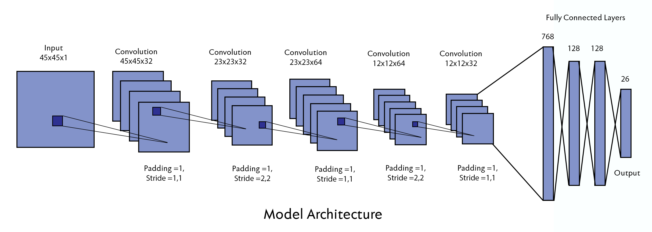

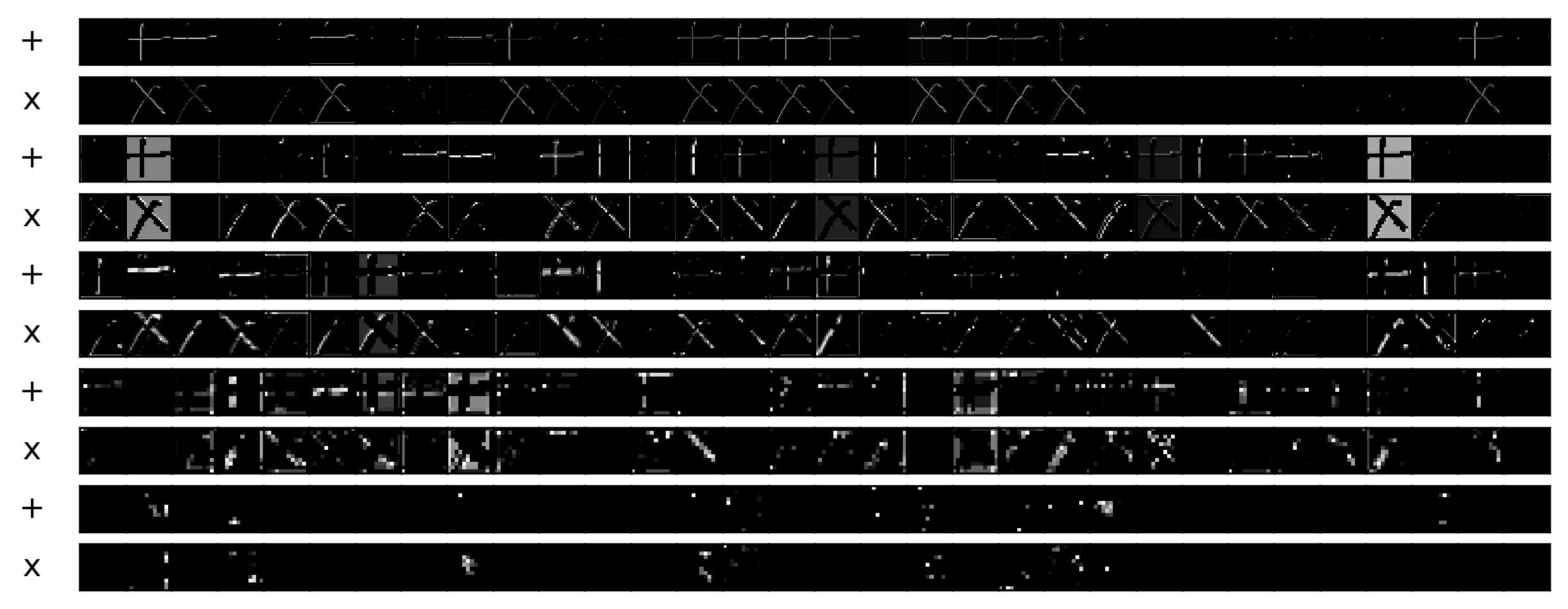
Before going to the evaluation , lets try to visualize how Convolutional layers really work

This is what the output from the 2nd convolutional layer looks like:

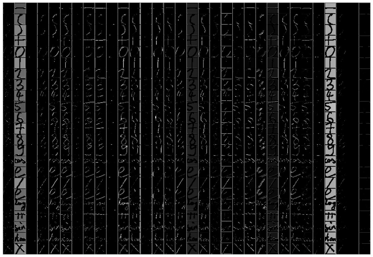
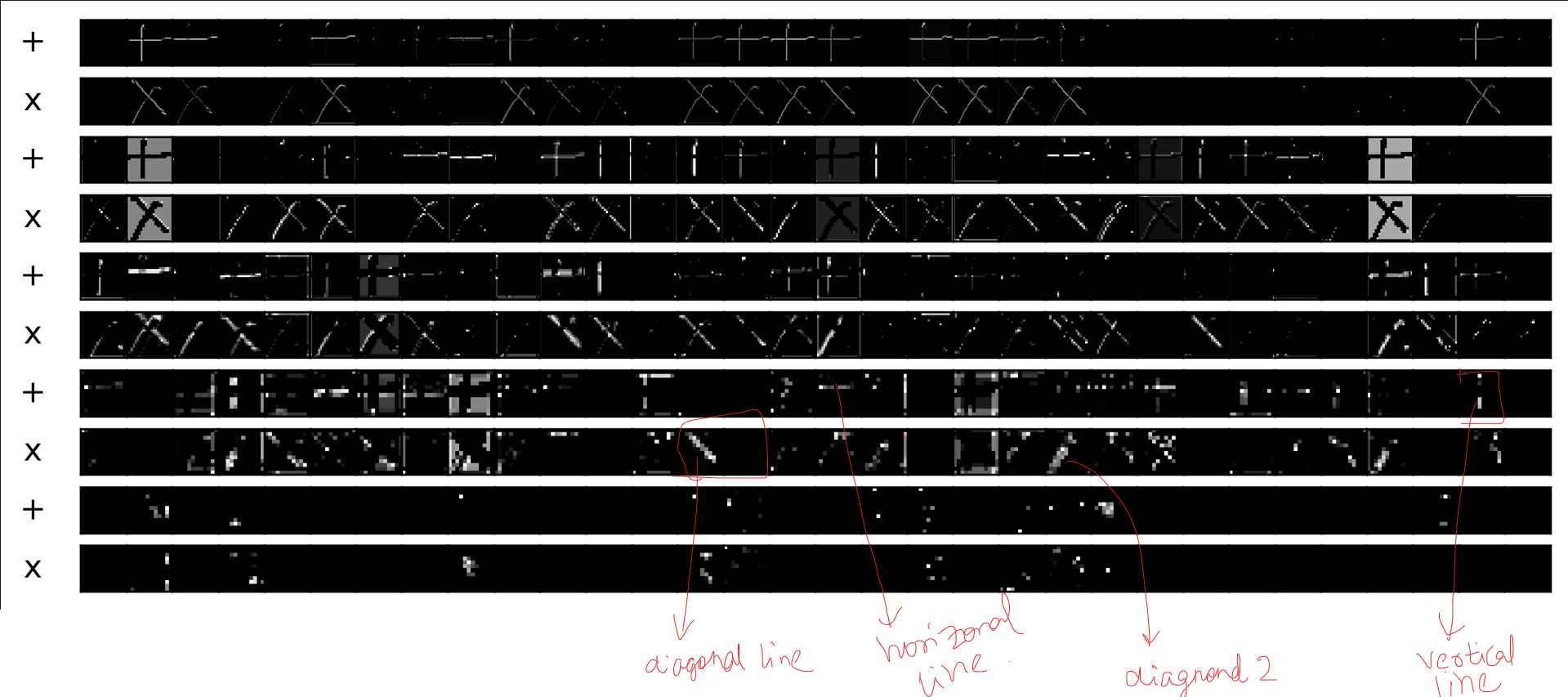
Lets take an example of + and x symbols and try to understand how the convolutional layer are

If we observe the 4th convolutional layer , we can see how the is detecting the slat line with this particular filter , as it is detecting a diagonal in the x and nothing for the + symbol.

Training and Evaluation

After training the model, we evaluated its performance using various metrics like accuracy and loss. Below are the training statistics and the confusion matrix.

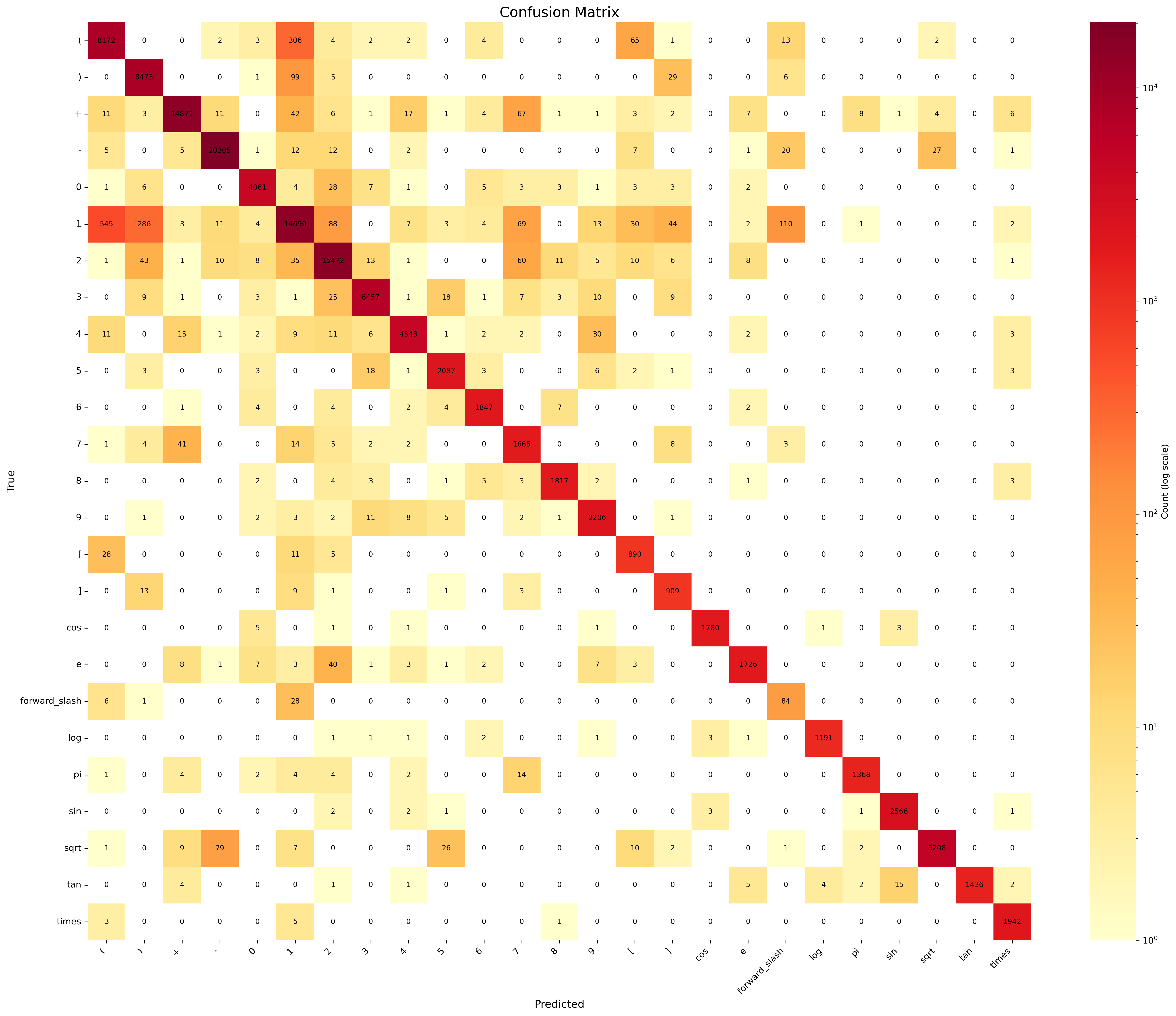
Dataset was not very good hence the model does perform well in the validation set , but it performs decently good with real life data , Hence we will move ahead with this model.

Solving the Equation

With our model ready to classify individual mathematical symbols, we now focus on solving the entire equation. This involves segmenting the image to isolate each symbol.

• Image Segmentation with OpenCV: Using OpenCV, we can detect and crop individual symbols from the equation image. Here are some key techniques used:

• Filters: To enhance image features. Bounding Boxes: To identify and isolate symbols.
• Contours: To detect the boundaries of symbols.

Now that we have the model to classify the symbols given a single image of the symbol but the input we are going to receive will be the image of the whole equation.

We will have to crop the image into different sections containing single symbols then input these image to our model.

this technique of cropping the image based on the requirement is known as image segmentation

First we import the image then we convert it to grayscale , after converting to grayscale we apply adaptiveThreshold to the image , based on the contours generated from the image the bounding boxes are generated

Interpreting and Solving the Equation

After segmenting the image and recognizing the symbols, we convert the sequence into a mathematical expression.

For this I created a class in python “Mathsymbol“ library helps in parsing and evaluating these expressions.

However, we must handle certain complexities , that we need to handle with the help of the custom class that we created:

Powers: Correctly parsing and solving expressions with exponents.

For example for the above image our model after doing the image segmentation will give this output,

['1', '-', '2', '+', '4', '3', '-', '9']

we will have to somehow mention that the 3 was raised to the power of 4. For this we can do one thing , notice how the vertical position of the digits that are raised to the power will be lower that compared to the rest of the symbols

Using this logic we label all the symbols as either pow or gr , pow for the symbols that are raised to the power

Hence the equation becomes from this to 
['1', '-', '2', '+', '4', '3', '-', '9']
this -> 1-2+4**3-9

Multiple Digits: Properly identifying and combining multiple digits.

For example for the above image our model after doing the image segmentation will give this output,

look how the 9,6 in 96 and 4,9 in 49 are separated to combine the digits we will use a simple logic that if the combine all the adjacent number if they have the same symbol type (either pow or gr)

['9', '6', '+', '(', '4', '9', '-', 'sqrt', 'e', ')', 'forward_slash', '2']
['96', '+', '(', '49', '-', 'sqrt', 'e', ')', 'forward_slash', '2']

final eq is  96+(49-math.sqrt(math.e))/2
final ans is  119.67563936464994

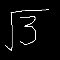
Square Roots: Accurately interpreting square root symbols.

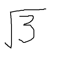
Consider this image

This is the output we will get , now we need to mention which symbols are to be considered inside the square root , for this we simply consider all the symbols that fall under the x coordinate of the square root to be inside the square root , hence in the above equation 16+9 will come under the square root

From this 
['9', '3', '+', 'sqrt', '1', '6', '+', '9', '-', '7', '2']
 we get this -> 93+math.sqrt(16+9)-7**2

Conclusion

By combining convolutional neural networks for symbol recognition with image segmentation techniques, we can build an efficient system for solving handwritten mathematical equations. This project showcases the power of machine learning in automating complex tasks and has practical applications in educational tools, digitizing handwritten notes, and more.

Thank you for reading! Feel free to explore the code and dataset linked above, and happy coding!